Structured Product Evaluation • Morgan Stanley Finance LLC • CUSIP 61781LZW3

Structured Product Evaluation Report

Worst-of EURO STOXX 50 / Russell 2000 / S&P 500 — Contingent Income Auto-Callable Notes due Nov 2, 2029

Headline Simulation Results 10,000 Monte-Carlo scenarios

8.90%

Expected annualized return

Mean of per-scenario annualized return

6.94%

Expected total return

Over the realized holding period (~1.06 y)

4.51%

Probability of a negative return

Chance of any loss at maturity

-17.37%

99% confidence VaR

1-year, 1st percentile

~1.06 y

Expected holding period

≈ 12.77 months

87.58%

Probability of automatic early redemption

Note called before maturity

Headline Metric	Value
Expected annualized return (mean of per-scenario annualized return)	8.90%
Expected total return over realized holding period	6.94%
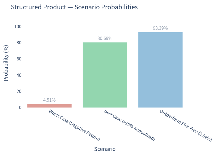
Probability of a negative return	4.51%
99% confidence VaR (1-year, 1st percentile)	-17.37%
Expected holding period	~1.06 years (12.77 months)
Probability of automatic early redemption	87.58%

Reading the annualized figure The note lives only ~1.06 years on average, and ~54% of scenarios are redeemed at the first call date (month 6). Short holding periods are annualized linearly (×12/months), which inflates the mean of per-scenario annualized returns to 8.90% versus a 6.94% expected total return over the ~1.06-year average life. Always read the annualized figure together with the total return and the holding period.

Basic Product Information

Issuer / Guarantor: Morgan Stanley Finance LLC / Morgan Stanley (USD, $1,000 per note).
Underlyings: EURO STOXX 50® Index (SX5E), Russell 2000® Index (RTY), S&P 500® Index (SPX). All payoff conditions depend on the worst-performing of the three.
Contingent coupon: 10.05%–11.05% p.a. (modeled at the 10.55% midpoint, ≈2.64 points per quarter), paid quarterly only if the worst-of level is at or above 80% of its starting level on the observation date.
Automatic early redemption: beginning after 6 months, then quarterly — if all three indices close at or above 100% of their starting levels, the note is called at par plus the period's coupon.
Downside protection: at maturity, if the worst-of final level is at or above 70% of its starting level, principal is returned in full; below 70%, principal is reduced 1:1 with the worst index (e.g. worst at 60% ⇒ 60% of principal returned).
Upside: capped — investors never participate in index appreciation.

How it works (plain language)

You put up $1,000. Every quarter you collect an attractive coupon (~2.64% of principal) as long as none of the three indices has dropped below 80% of where it started. Starting after six months, the note is called away automatically (you get your $1,000 back plus that quarter's coupon) as soon as all three indices are back to at least their starting levels. If the note survives to 2029, you get your full $1,000 back provided the weakest index is still above 70% of its start; if the weakest index falls below 70%, you lose principal one-for-one with that decline. Upside is capped at par plus coupons, but downside below the 70% barrier on the worst index is effectively uncapped down to −100%.

Key Statistics — Structured Product vs Underlying Benchmark

Benchmark = buy-and-hold of an equal-weight basket of the three indices over the full 3-year term, total return including an average dividend yield of ≈1.56%. This unconditional measure is the fair "standalone investment" reference.

Metric	Structured Product	Underlying (Buy & Hold 3y, Total Return)
Expected annualized return	8.90%	10.39%
Expected annualized volatility	5.26%	9.86%
Probability of loss	4.51%	18.22%
99% VaR (1 year)	-17.37%	-14.68%
Expected total return (over its horizon)	6.94% (over ~1.06 y)	32.07% (over 3 y)

3.84%

Risk-free rate

1-year U.S. T-bill average

93.39%

Probability of beating the risk-free rate

Note annualized return vs 3.84% T-bill

80.69%

Probability of annualized return above 10%

Below the autocall probability

Why is the "above 10%" probability lower than the autocall probability? A fixed ≈2.64%/quarter coupon compounds to under 10.55% p.a. on multi-year holds — later calls at months 27/30/33 earn only ~9.7–9.9% annualized even with every coupon — and a few early calls skip an earlier coupon after a sub-80% quarterly print.

Comparison summary

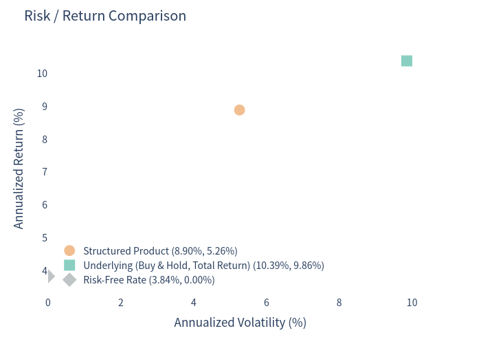
Versus simply buying and holding the basket, the note delivers a lower expected return (8.90% vs 10.39%) and carries a deeper 99% tail (-17.37% vs -14.68%) because its payoff is tied to the weakest index, but it offers far lower volatility (5.26% vs 9.86%) and a much smaller chance of any loss (4.51% vs 18.22%) thanks to the 70% barrier and the coupon cushion.

Charts

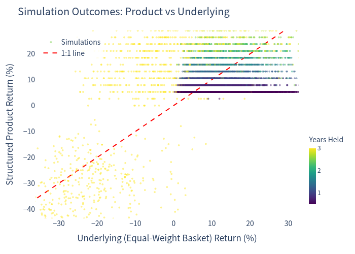
Simulation outcomes: product vs underlying (same realized holding period)

Each dot is one of the 10,000 scenarios. The x-axis measures the equal-weight basket over the same realized holding period as the note, so it captures the per-scenario opportunity cost; colour marks how long the note was held. Because upside is capped, product returns sit in a tight band around par-plus-coupon, while deep drawdowns of the worst index pull product returns sharply negative.

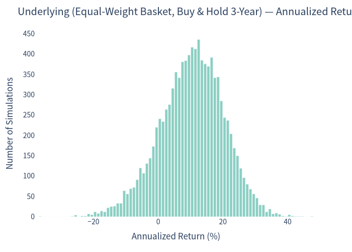
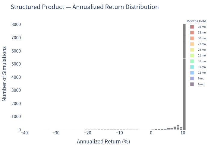
Scatter plot of product vs underlying outcomes over the same realized holding period

Product vs underlying basket outcomes — per-scenario scatter

Annualized return distributions

The buy-and-hold basket has a broad, right-skewed distribution with meaningful left tail; the product distribution is compressed near the coupon level with a thin negative tail coming from maturity barrier breaches (and stacking by holding period shows most mass at the early-call level).

Histogram of annualized returns for the underlying buy-and-hold basket

Underlying basket — annualized return distribution

Histogram of annualized returns for the structured product

Structured product — annualized return distribution

Risk vs return

The note sits to the left of the buy-and-hold basket — much lower volatility and a lower expected return — while its deep tail (VaR) is somewhat worse.

Risk vs return — product compared with the underlying basket

Return box plot

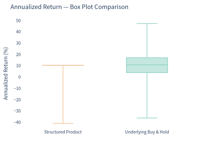
Most product outcomes cluster at the maximum coupon-driven level (~10.5% annualized, after an early call); the box plot contrasts this tight, callable profile with the much wider standalone basket.

Return distribution box plot

Scenario probabilities

Holding period and coupon distributions

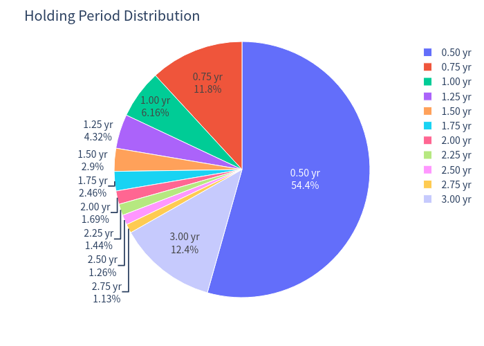
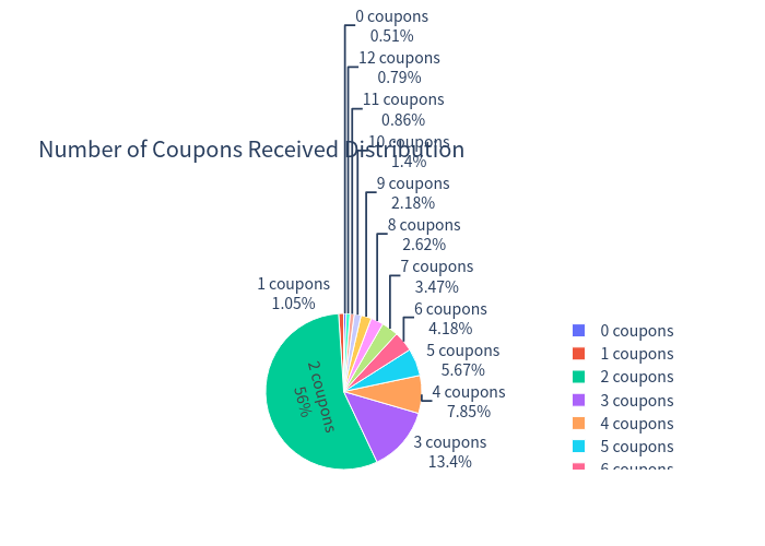
Automatic redemption concentrates outcomes into a first call at month 6 (~54%) and a full-term survival (~12%).

Holding period distribution

Coupons received distribution

Investment Commentary

Potential advantages

High headline coupon (~10.55% p.a.), paid whenever the worst-of index is above 80% of its start — a level the worst index clears in the large majority of quarterly observations.
Frequent early redemption — ~88% of scenarios are called, most at the first opportunity, returning principal quickly with several coupons.
Downside buffer to −30% on the worst-of index lowers the probability of any loss to ≈4.5% (versus ≈18% for a buy-and-hold basket) and keeps volatility low (~5%).
Attractive risk-adjusted profile — a ~93% probability of beating the 1-year T-bill and a substantially lower chance of loss than holding the indices directly.

Considerations / trade-offs

Capped upside: investors forgo index appreciation; in strong markets the note is simply called and must be reinvested, possibly at lower future rates.
Worst-of exposure: returns are tied to the weakest of three indices, so one lagging market can trigger a loss even if the others rise. This is why the note's 99% VaR (-17.37%) is worse than the diversified basket (-14.68%) despite its much lower volatility.
Lower expected return: the coupon-rich, callable, barrier structure buys its reduced risk at the cost of a lower expected return than plain index exposure (8.90% vs 10.39% annualized).
Call / reinvestment and credit risk: a ~1-year expected life means proceeds may need reinvesting at unknown rates, and payments depend on Morgan Stanley's creditworthiness.

All figures are model-based estimates from a 36-month Monte-Carlo simulation and are provided for information only; they are not a recommendation or suitability assessment.