
Contingent Income Auto-Callable Securities — Simulation Report
1. Headline Simulation Results
Based on 10,000 Monte Carlo simulations over the 36-month term (inferred quarterly observation schedule; contingent coupon assumed at the midpoint of the 10.25%–11.25% range = 10.75% p.a.):
| Headline metric | Structured Product |
|---|---|
| Expected annualized return | 8.92% |
| Expected total return over the holding period | 7.15% |
| Probability of a negative return | 4.95% |
| 99% confidence 1-year VaR | −17.35% |
| Expected annualized volatility | 5.47% |
| Expected holding period | 13.3 months (median 6 months) |
| Probability of early autocall | 86.0% |
The structure produces a high probability of a modest, capped gain, at the cost of a small but severe downside tail. Roughly 4.95% of paths deliver a negative total return, and the loss in the worst 1% of simulations reaches an annualized −17.35% (the security can lose up to its full principal).
2. How the Product Works (in plain terms)
This is a 3-year “worst-of” autocallable note linked to three equity indices: the Dow Jones Industrial Average, the EURO STOXX 50 and the Russell 2000.
- Contingent coupon (≈10.75% p.a., quarterly): On each quarterly observation date you receive a coupon only if all three indices are at or above 80% of their starting level. If any index is below 80%, that quarter’s coupon is lost (no accrual, no catch-up).
- Automatic early redemption (from month 6): If on a quarterly redemption-determination date all three indices are back at or above 100% of their start, the note is called immediately and you receive par plus the period’s coupon.
- Principal at risk at maturity: If never called, you get par back only if all three indices finish at or above 70% of their start. If any index finishes below 70%, you lose 1% of principal for every 1% that the worst-performing index fell. The payment can be as low as zero.
- Upside is capped: You do not participate in index appreciation beyond the coupons.
Because the payoff is driven by the worst of the three indices, the diversification benefit of holding three markets is removed — the weakest market dictates the outcome.
3. Key Statistics
| Metric | Structured Product | Benchmark (equal-weight basket, total return*) |
|---|---|---|
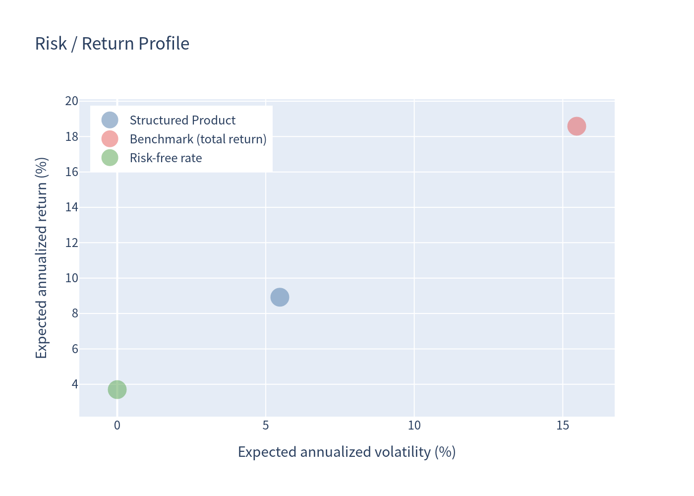
| Expected annualized return | 8.92% | 18.58% |
| Expected annualized volatility | 5.47% | 15.47% |
| Probability of loss | 4.95% | 9.41% |
| 99% VaR (1 year) | −17.35% | −12.58% |
| Expected total return (holding period) | 7.15% | 9.92% |
Interpreting the annualized benchmark figure: the product is typically redeemed early and only when all three markets are up, so the benchmark is compared over these same, mostly short and state-dependent windows. Annualizing short positive returns (e.g. a 6-month gain × 2) mechanically inflates the benchmark’s expected annualized number. On a like-for-like total-return basis the gap is smaller (product 7.15% vs basket 9.92%), and the product achieves it with roughly one-third of the volatility.
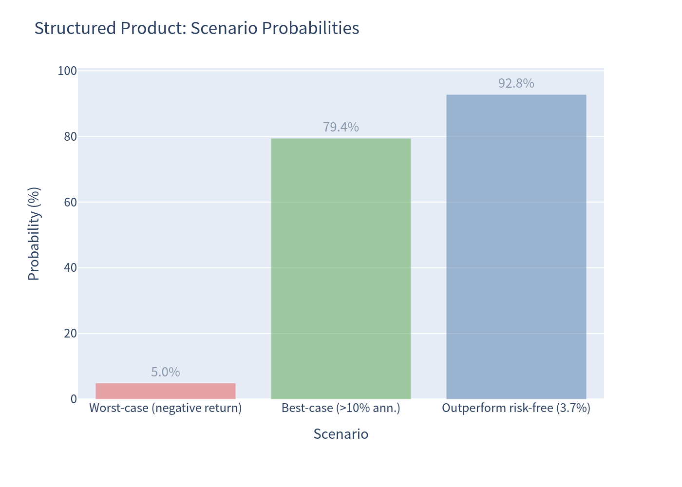
Scenario probabilities (structured product)
| Scenario | Probability |
|---|---|
| Worst-case — negative total return | 4.95% |
| Best-case — annualized return above 10% | 79.44% |
| Outperforms the risk-free rate (3.70%) | 92.77% |
The maximum possible outcome is a full 12 quarters of coupons plus par = 132.25 index points (+32.25%).
4. Charts
4.1 Simulation outcomes — product vs benchmark
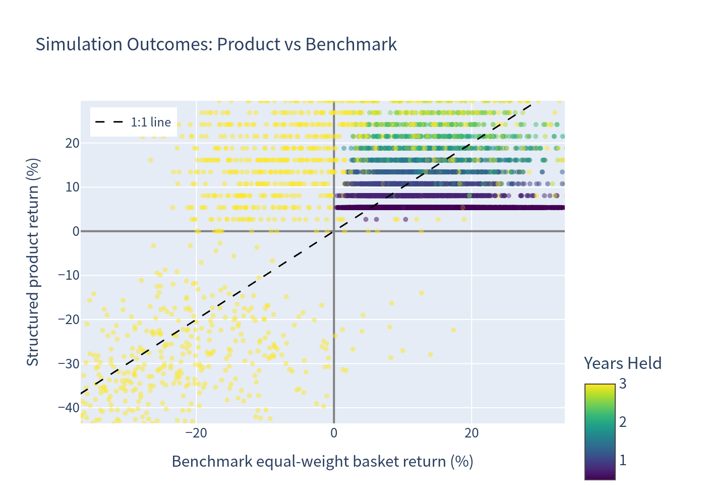
Each point is one simulation; colour = number of years held; dashed line is the 1:1 line. The product’s returns are clustered at a capped ceiling (coupons + par) while outcomes fall sharply once the worst index breaches the 70% barrier.
4.2 Annualized-return histograms (1% bins, stacked by holding period)
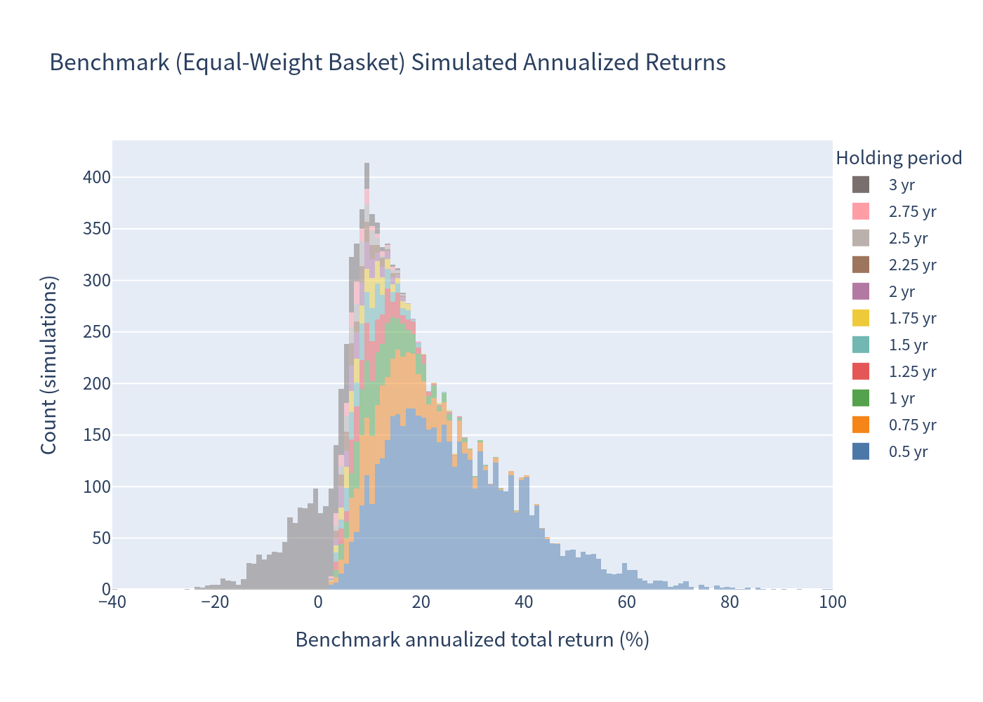
Benchmark (equal-weight basket, total return)
Structured product
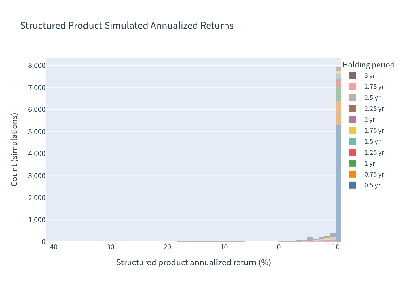
The product’s distribution is a tall spike near +10.75% (coupons collected and principal returned) with a thin negative tail — the mirror image of the benchmark’s wide, symmetric spread.
4.3 Risk / return profile
4.4 Annualized-return box plot
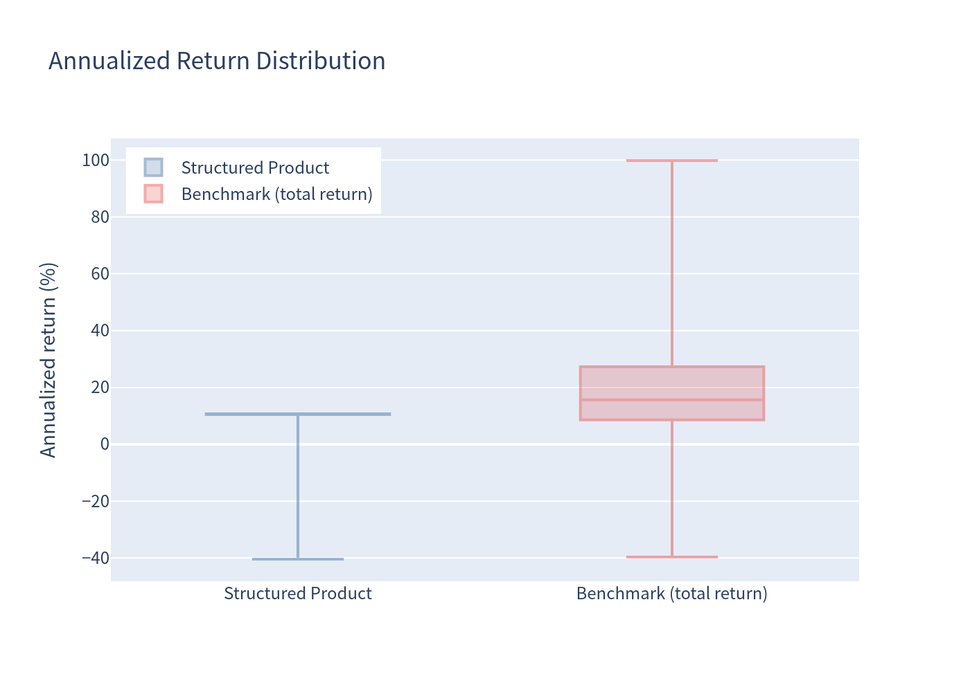
4.5 Scenario probabilities
4.6 Holding-period and coupon-count distribution
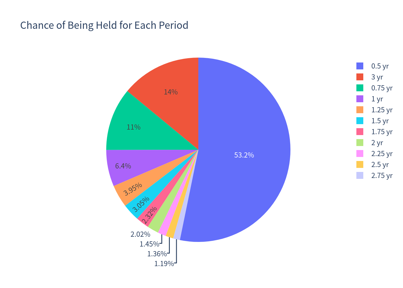
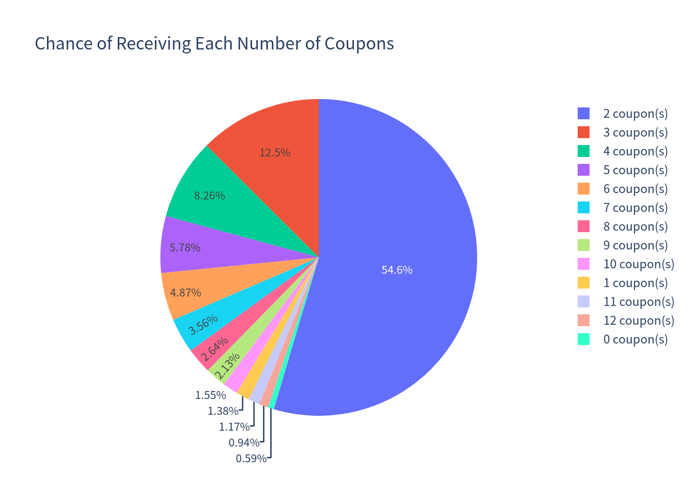
The note is called within the first year in ~70% of simulations (about 53% at the very first call date, month 6). The most common outcome is 2 coupons (≈54.6% of paths).
5. Investment Commentary
Potential merits
- Above-market contingent yield: an assumed ~10.75% p.a. coupon is attractive versus prevailing 1-year T-bill rates of ~3.7%.
- Frequent, quick outcomes: ~86% of paths autocall early, with an expected holding period of ~13 months — capital is returned and can be redeployed quickly in the base case.
- High hit-rate on the income: 92.77% of simulations beat the risk-free rate and ~79% deliver more than 10% annualized.
- Lower measured volatility than the equity basket (5.47% vs 15.47%), reflecting the coupon cushion and the barrier structure.
Key risks to weigh
- Capped upside: no participation in index gains beyond the coupons (max +32.25% over the full term).
- Worst-of exposure: the single weakest of three indices drives both coupon eligibility and the redemption amount; a sharp fall in one market is enough to wipe out the coupon or principal.
- Principal at risk: below the 70% downside threshold the note loses 1:1 with the worst index, and the 99% VaR (−17.35%) is worse than the benchmark’s — the loss tail is fatter even though the typical outcome is far more stable.
- No coupon if the 80% barrier is breached on any observation date; coupons already skipped are not recovered later.
- Credit and liquidity risk: the note is an unsecured Morgan Stanley/MSFL obligation and is not listed.